causal effect analysis

we could be able to analyze whether one variable have an impact on another variable

linear fitting

import tensorflow as tf
linear_model = tf.keras.Sequential([
    layers.Dense(units=1, use_bias=False)
])
linear_model.compile(
    optimizer=tf.optimizers.Adam(learning_rate=0.1),
    loss=tf.keras.losses.MeanSquaredError()
)
linear_model.fit(
    df[['Operation']],
    df['Sales'],
    epochs=100,
    verbose=0,
)
linear_model.get_weights()

TensorFlow Probability

Bayesian Structural Time Series

by simulating control group and computing the difference we can analyze the causal effect. the bsts algorithm is able to model a wild range of possibilities while offering Bayesian priors.

models

AutoRegressive: Each new state space point receives a value that is a linear combination of the previous components.
Dynamic Regression: Adds a component that is a linear combination of covariates that further help explain the observed data. The dynamic part is implemented through the addition of a Gaussian random walk.
LocalLevel: Represents essentially a random walk. This component will be used as default by tfcausalimpact later on as it works as an exchange between how well our covariates explain the data or how much the random walk dominates the state space which means the observed data behaves like random fluctuation over time.
Seasonal: Models patterns that repeat over time such as weekly or daily seasons.
LocalLinearTrend: Similar to local level but it adds another slope component which models a constantly increasing (or decreasing) pattern from data.
SemiLocalLinearTrend: Similar to local linear trend but the slope model follows an auto regressive component of first order.
SmoothSeasonal: Also models seasonal effects, this time specified in terms of multiples of a base frequency.

example

#combi model of local level with a linear regression
import numpy as np
import pandas as pd
import matplotlib.pyplot as plt
import tensorflow_probability as tfp


x = np.random.rand(30)
y = 2.2 * x + np.random.rand(30)
data = pd.DataFrame({'X': x, 'y': y}, dtype=np.float32)
obs_data = data['y'].iloc[:20]

level = tfp.sts.LocalLevel(observed_time_series=obs_data)
linear = tfp.sts.LinearRegression(design_matrix=data['X'][..., np.newaxis])
model = tfp.sts.Sum([level, linear], observed_time_series=obs_data)

samples, _ = tfp.sts.fit_with_hmc(model, obs_data)

dist = tfp.sts.forecast(model, obs_data, samples, 10)
mean, std = dist.mean(), dist.stddev()

fig = plt.figure(figsize=(12, 10))
ax = plt.subplot(1, 1 ,1)
ax.plot(np.arange(30), data['X'], label='X', lw=1)
ax.plot(np.arange(30), data['y'], label='y', lw=2, color='orangered')
ax.scatter(np.arange(30), data['y'], lw=2, color='red')
ax.plot(np.arange(20, 30), mean, color='k', ls='--', label='forecast mean')
ax.fill_between(np.arange(20, 30), np.squeeze(mean - 1.96 * std),
                np.squeeze(mean + 1.96 * std), color='orange', alpha=0.3,
                label='95% CI')
plt.legend(loc='best')

tfcausalimpact

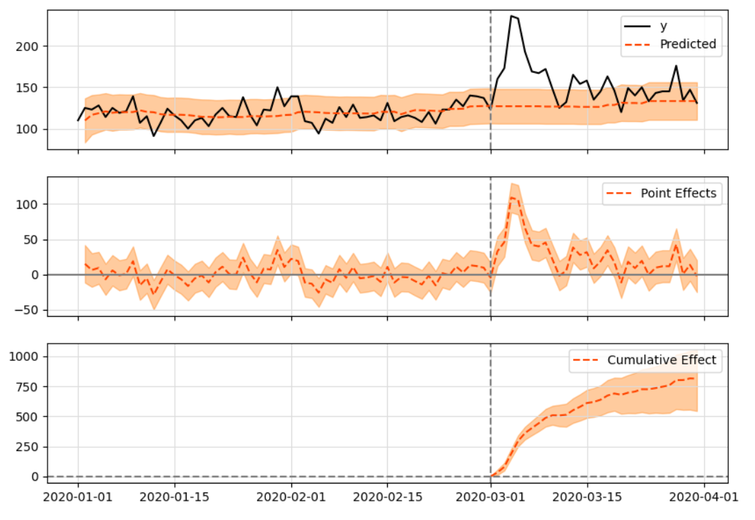
this model is appropriate for impacts that are expected to last a few data points into the future and then fades away

import pandas as pd
from causalimpact import CausalImpact

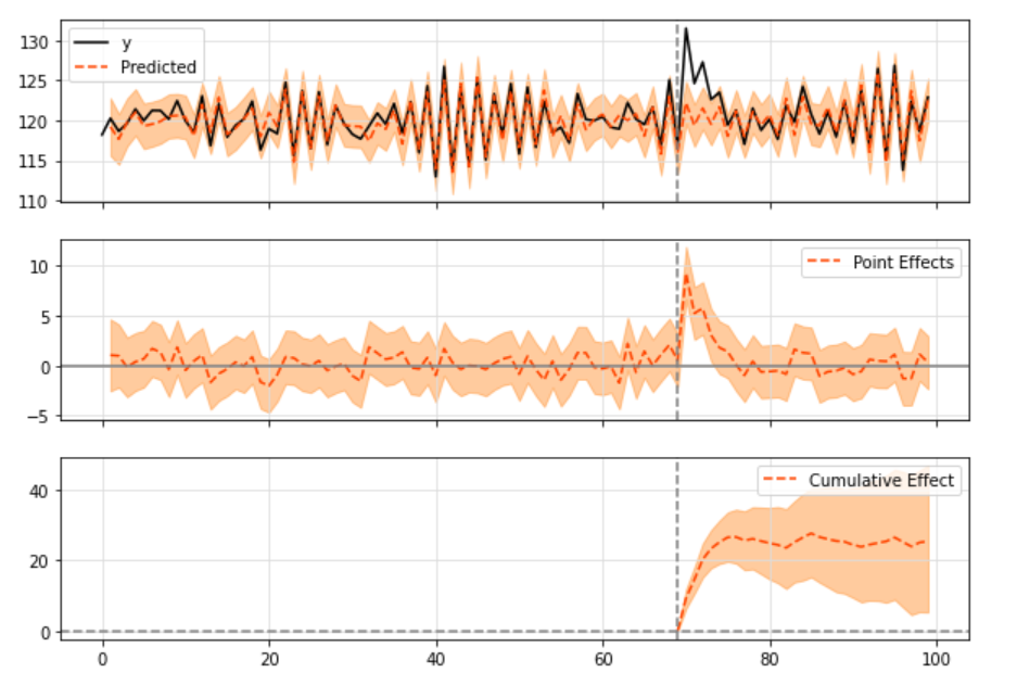
data = pd.read_csv('https://raw.githubusercontent.com/WillianFuks/tfcausalimpact/master/tests/fixtures/arma_data.csv')[['y', 'X']]
data.iloc[70:77, 0] += np.arange(7, 0, -1)
pre_period = [0, 69]
post_period = [70, 99]

#use default model
ci = CausalImpact(data, pre_period, post_period)
print(ci.summary())
ci.plot()

#use customized model
import tensorflow_probability as tfp
from causalimpact.misc import standardize


normed_data, mu_sig = standardize(data)
obs_data = normed_data['BTC-USD'].loc[:'2020-10-14'].astype(np.float32)
design_matrix = pd.concat(
    [normed_data.loc[pre_period[0]: pre_period[1]], normed_data.loc[post_period[0]: post_period[1]]]
).astype(np.float32).iloc[:, 1:]
linear_level = tfp.sts.LocalLinearTrend(observed_time_series=obs_data)
linear_reg = tfp.sts.LinearRegression(design_matrix=design_matrix)
month_season = tfp.sts.Seasonal(num_seasons=4, num_steps_per_season=1, observed_time_series=obs_data, name='Month')
year_season = tfp.sts.Seasonal(num_seasons=52, observed_time_series=obs_data, name='Year')
model = tfp.sts.Sum([linear_level, linear_reg, month_season, year_season], observed_time_series=obs_data)

ci = CausalImpact(data, pre_period, post_period, model=model)

# use different backend algo
from causalimpact import CausalImpact
pre_period=[‘2018–01–03’, ‘2020–10–14’]
post_period=[‘2020–10–21’, ‘2020–11–25’]
ci = CausalImpact(data, pre_period, post_period, model_args={‘fit_method’: ‘hmc’})

model decomposition analysis

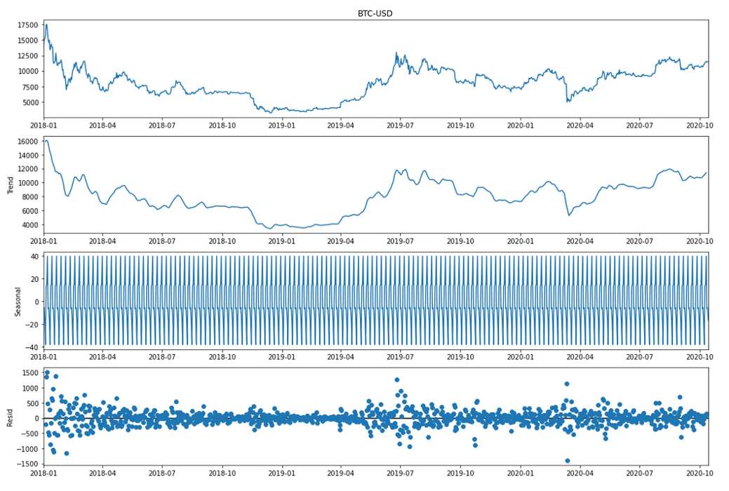
from statsmodels.tsa.seasonal import seasonal_decompose
result = seasonal_decompose(btc_data.loc[:’2020–10–14'].iloc[:, 0])
result.plot();

Related Issues not found

Please contact @neverset123 to initialize the comment