Support vector machines (SVM) is a supervised machine learning. Application areas include:
- classification
- regression
Its biggest advantage is that it can define both a linear or a non-linear decision boundary by using kernel functions.
support vector machines also draws a margin around the decision boundary to increase prediction confidence.
Support vector machines allow some misclassification during the learning process. So they can do a better job at classifying most vectors in the testing set.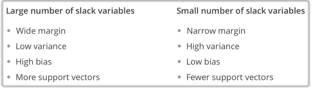
usage
    import random
    import numpy as np
    import pandas as pd
    import matplotlib.pyplot as plt
    def generate_random_dataset(size):
    """ Generate a random dataset and that follows a quadratic  distribution
    """
    x = []
    y = []
    target = []
    for i in range(size):
            # class zero
            x.append(np.round(random.uniform(0, 2.5), 1))
            y.append(np.round(random.uniform(0, 20), 1))
            target.append(0)
            # class one
            x.append(np.round(random.uniform(1, 5), 2))
            y.append(np.round(random.uniform(20, 25), 2))
            target.append(1)
            x.append(np.round(random.uniform(3, 5), 2))
            y.append(np.round(random.uniform(5, 25), 2))
            target.append(1)
    df_x = pd.DataFrame(data=x)
    df_y = pd.DataFrame(data=y)
    df_target = pd.DataFrame(data=target)
    data_frame = pd.concat([df_x, df_y], ignore_index=True, axis=1)
    data_frame = pd.concat([data_frame, df_target], ignore_index=True, axis=1)
    data_frame.columns = ['x', 'y', 'target']
    return data_frame

    # Generate dataset
    size = 100
    dataset = generate_random_dataset(size)
    features = dataset[['x', 'y']]
    label = dataset['target']
    # Hold out 20% of the dataset for training
    test_size = int(np.round(size * 0.2, 0))
    # Split dataset into training and testing sets
    x_train = features[:-test_size].values
    y_train = label[:-test_size].values
    x_test = features[-test_size:].values
    y_test = label[-test_size:].values
    # Plotting the training set
    fig, ax = plt.subplots(figsize=(12, 7))
    # removing to and right border
    ax.spines['top'].set_visible(False)
    ax.spines['left'].set_visible(False)
    ax.spines['right'].set_visible(False)
    # adding major gridlines
    ax.grid(color='grey', linestyle='-', linewidth=0.25, alpha=0.5)
    ax.scatter(features[:-test_size]['x'], features[:-test_size]['y'], color="#8C7298")
    plt.show()

    #train model
    from sklearn import svm
    model = svm.SVC(kernel='poly', degree=2)
    model.fit(x_train, y_train)

    #plot decision boundary
    fig, ax = plt.subplots(figsize=(12, 7))
    # Removing to and right border
    ax.spines['top'].set_visible(False)
    ax.spines['left'].set_visible(False)
    ax.spines['right'].set_visible(False)
    # Create grid to evaluate model
    xx = np.linspace(-1, max(features['x']) + 1, len(x_train))
    yy = np.linspace(0, max(features['y']) + 1, len(y_train))
    YY, XX = np.meshgrid(yy, xx)
    xy = np.vstack([XX.ravel(), YY.ravel()]).T
    train_size = len(features[:-test_size]['x'])
    # Assigning different colors to the classes
    colors = y_train
    colors = np.where(colors == 1, '#8C7298', '#4786D1')
    # Plot the dataset
    ax.scatter(features[:-test_size]['x'], features[:-test_size]['y'], c=colors)
    # Get the separating hyperplane
    Z = model.decision_function(xy).reshape(XX.shape)
    # Draw the decision boundary and margins
    ax.contour(XX, YY, Z, colors='k', levels=[-1, 0, 1], alpha=0.5, linestyles=['--', '-', '--'])
    # Highlight support vectors with a circle around them
    ax.scatter(model.support_vectors_[:, 0], model.support_vectors_[:, 1], s=100, linewidth=1, facecolors='none', edgecolors='k')
    plt.show()

    #run test
    from sklearn.metrics import accuracy_score
    predictions_poly = model.predict(x_test)
    accuracy_poly = accuracy_score(y_test, predictions_poly)
    print("2nd degree polynomial Kernel\nAccuracy (normalized): " + str(accuracy_poly))