network visualization is used to do social network analysis.
network theory
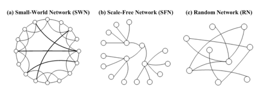
- small world: real networks often have very short paths (in terms of number of hops) between any connected network members.
- scale free network: a skewed population with a few highly-connected nodes (such as social-influences) and a lot of loosely-connected nodes
- homophily: tendency of individuals to associate and bond with similar others, which results in similar properties among neighbors
Centrality
- Degree — the amount of neighbors of the node
- EigenVector / PageRank — iterative circles of neighbors
- Closeness — the level of closeness to all of the nodes
- Betweenness — the amount of short path going through the node
Different measures can be useful in different scenarios such as web-ranking (page-rank), critical points detection (betweenness), transportation hubs (closeness)
build network graph
networkx
built-in graph in networkx
votes_data = pd.read_excel('ESC2018_GF.xlsx',sheetname='Combined result')

votes_melted = votes_data.melt(
    ['Rank','Running order','Country','Total'],
    var_name = 'Source Country',value_name='points')

G = nx.from_pandas_edgelist(votes_melted,
                            source='Source Country',
                            target='Country',
                            edge_attr='points',
                            create_using=nx.DiGraph())

nx.draw_networkx(G)
customized graph
countries = pd.read_csv('countries.csv',index_col='Country')

pos_geo = {  node:
        ( max(-10,min(countries.loc[node]['longitude'],55)), # fixing scale
            max(countries.loc[node]['latitude'],25)) #fixing scale
            for node in G.nodes() }
            pos_geo = {}

for node in G.nodes():
    pos_geo[node] = (
                    max(-10,min(countries.loc[node]['longitude'],55)), # fixing scale
                    max(countries.loc[node]['latitude'],25) #fixing scale  )

flags = {}
flag_color = {}
for node in tqdm.tqdm_notebook(G.nodes()):
    flags[node] = 'flags/'+(countries.loc[node]['cc3']).lower().replace(' ','')+'.png'
    flag_color[node] =  ColorThief(flags[node]).get_color(quality=1)

def RGB(red,green,blue):
    return '#%02x%02x%02x' % (red,green,blue)

ax=plt.gca()
fig=plt.gcf()
plt.axis('off')
plt.title('Eurovision 2018 Final Votes',fontsize = 24)

trans = ax.transData.transform
trans2 = fig.transFigure.inverted().transform

tick_params = {'top':'off', 'bottom':'off', 'left':'off', 'right':'off',
            'labelleft':'off', 'labelbottom':'off'} #flag grid params

styles = ['dotted','dashdot','dashed','solid'] # line styles

pos = pos_geo

# draw edges
for e in G.edges(data=True):
    width = e[2]['points']/24 #normalize by max points
    style=styles[int(width*3)]
    if width>0.3: #filter small votes
        nx.draw_networkx_edges(G,pos,edgelist=[e],width=width, style=style, edge_color = RGB(*flag_color[e[0]]) )
        # in networkx versions >2.1 arrowheads can be adjusted

#draw nodes
for node in G.nodes():
    imsize = max((0.3*G.in_degree(node,weight='points')
                /max(dict(G.in_degree(weight='points')).values()))**2,0.03)

    # size is proportional to the votes
    flag = mpl.image.imread(flags[node])

    (x,y) = pos[node]
    xx,yy = trans((x,y)) # figure coordinates
    xa,ya = trans2((xx,yy)) # axes coordinates

    country = plt.axes([xa-imsize/2.0,ya-imsize/2.0, imsize, imsize ])
    country.imshow(flag)
    country.set_aspect('equal')
    country.tick_params(**tick_params)

fig.savefig('images/eurovision2018_map.png')
hypergraph
star expansion
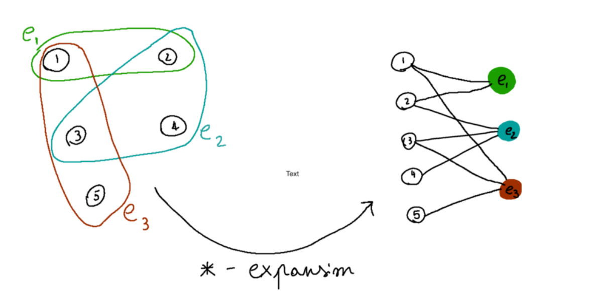 a new graph having as node set both the nodes and the edges of the original hypergraph is created, and the edges are given by the incidence relations in the original hypergraph (if a node n was part of an edge e in the hypergraph, there should be an edge between n and e in the new graph).
decompose hypergraph into many graphs
decompose the edges of a hypergraph by how many nodes they contain into 2-body interactions, 3-body interactions, and so on.
```from collections import defaultdict
def decompose_edges_by_len(hypergraph): decomposed_edges = defaultdict(list) for edge in hypergraph[‘edges’]: decomposed_edges[len(edge)].append(edge) decomposition = { ‘nodes’: hypergraph[‘nodes’], ‘edges’: decomposed_edges } return decomposition
import networkx as nx from networkx import NetworkXException import matplotlib.pyplot as plt
def plot_hypergraph_components(hypergraph): decomposed_graph = decompose_edges_by_len(hypergraph) decomposed_edges = decomposed_graph[‘edges’] nodes = decomposed_graph[‘nodes’]
n_edge_lengths = len(decomposed_edges)

# Setup multiplot style
fig, axs = plt.subplots(1, n_edge_lengths, figsize=(5*n_edge_lengths, 5))
if n_edge_lengths == 1:
    axs = [axs]  # Ugly hack
for ax in axs:
    ax.axis('off')
fig.patch.set_facecolor('#003049')

# For each edge order, make a star expansion (if != 2) and plot it
for i, edge_order in enumerate(sorted(decomposed_edges)):
    edges = decomposed_edges[edge_order]
    g = nx.DiGraph()
    g.add_nodes_from(nodes)
    if edge_order == 2:
        g.add_edges_from(edges)
    else:
        for edge in edges:
            g.add_node(tuple(edge))
            for node in edge:
                g.add_edge(node,tuple(edge))

    # I like planar layout, but it cannot be used in general
    try:
        pos = nx.planar_layout(g)
    except NetworkXException:
        pos = nx.spring_layout(g)

    # Plot true nodes in orange, star-expansion edges in red
    extra_nodes = set(g.nodes) - set(nodes)
    nx.draw_networkx_nodes(g, pos, node_size=300, nodelist=nodes,
                           ax=axs[i], node_color='#f77f00')
    nx.draw_networkx_nodes(g, pos, node_size=150, nodelist=extra_nodes,
                           ax=axs[i], node_color='#d62828')

    nx.draw_networkx_edges(g, pos, ax=axs[i], edge_color='#eae2b7',
                           connectionstyle='arc3,rad=0.05', arrowstyle='-')

    # Draw labels only for true nodes
    labels = {node: str(node) for node in nodes}
    nx.draw_networkx_labels(g, pos, labels, ax=axs[i])```
information flow
there are two basic models available to describe information flow process
- Linear Threshold: the influence accumulates from multiple neighbors of the node, which becomes activated only if the cumulative influence passed a certain threshold
-
Independent Cascade model: each of the node’s active neighbors has a probabilistic and independent chance to activate the node
def independent_cascade(G,t,infection_times): #doing a t->t+1 step of independent_cascade simulation #each infectious node infects neigbors with probabilty proportional to the weight max_weight = max([e[2][‘weight’] for e in G.edges(data=True)]) current_infectious = [n for n in infection_times if infection_times[n]==t] for n in current_infectious: for v in G.neighbors(n): if v not in infection_times: if G.get_edge_data(n,v)[‘weight’] >= np.random.random()*max_weight: infection_times[v] = t+1 return infection_times
infection_times = {‘Bran-Stark’:-1,’Samwell-Tarly’:-1,’Jon-Snow’:0}
for t in range(10): plot_G(subG,pos,infection_times,t) infection_times = independent_cascade(subG,t,infection_times)
Influence Maximization
influence maximization is to select a limited set of nodes in the network (seeding set) such that will naturally spread the influence to as much nodes as possible.
#find degree center
nx.degree(G, weight = None)
#find page-rank center
nx.pagerank_numpy(G, weight='weight')
#find weighted degree center
nx.degree(G, weight='weight')
#find betweenness center
nx.betweenness_centrality(G, weight='weight')